The solver for the maximum stable set problem uses branch & bound with a fixed clique partition for bounding. Minimum vertex covers are obtained by taking the complementary node set of a maximum stable set. Maximum cliques are obtained by computing maximum stable sets in complementary graphs. The latter is inefficient if the original graph is very sparse.
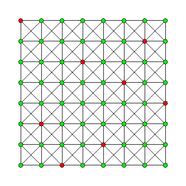
The following diagram shows an independent positioning of queens on a chess board. In the underlying graph, nodes are adjacent if they are on a common grid line or diagonal:

Bipartite graphs mean 2-colourable graphs. Probably the most famous theorem in graph theory states that every planar graph can be coloured with at most 4 different colours. The library comes up with a 5-colouring scheme for planar graphs. For the general setting, no efficient approximating method is available.
Observe that any clique size is a lower bound on the chromatic number (the minimum number of colour classes). If both numbers are equal and a maximum clique is given in advance (by the node colour register!), the node colour enumeration scheme will find a minimal colouring with some luck. Otherwise, only little effort is spent on computing a clique for dual bounding and it is most likely that the enumeration must be interrupted to obtain the heuristic solution found so far.
Similar to node colouring is the task of partitioning the node set into a minimum number of cliques. In the library, this problem is solved by searching for node colourings in the complementary graph. Needless to say that this is inefficient if the original graph is very sparse. If the graph is triangle free, however, clique partitioning is equivalent with maximum 1-matching, and this can be solved efficiently.
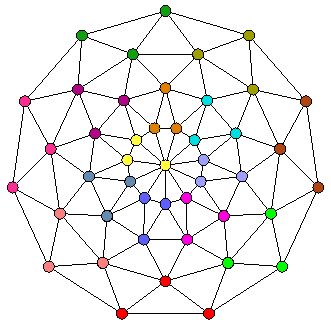
The following illustrates the clique cover problem. It is obvious that the displayed cover is minimal, since the graph does not include any 4-cliques (and this in turn follows from the fact that the graph is outerplanar):
The solver also applies to directed and even mixed graphs. To this end, let the bipartition distinguish into left-hand and right-hand nodes. The goal is to maximize the length of non-blocking arcs in the left-to-right direction.
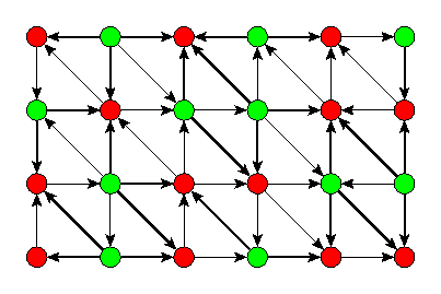
The following is a directed unit length and capacity example where the green nodes are left-hand and the red nodes are right-hand nodes:
There is no elaborate branch & bound scheme for this problem, but only a 1/2 approximation method which is pretty analugue of the max-cut approximation.
In principle, the library method for maximum tree packing also applies to the capacitated extension of this problem. But the procedure is only weakly polynomial, and the packing can be saved completely to the edge colour register only in the standard setting since a non-trivial capacity bound C means that this arc can be in C arborescences. The latter limitation can be overcome by using the extended API which allows to generate the arborescences step by step.
The procedure is little performant, and suited rather to illustrate the min-max relationship with minimum r-cut on small examples. Today, there is no method for the undirected analogue or even the extension to mixed graphs.
There is also a standard notation of f-factors which differ from perfect b-matchings by that one does not allow for edge multiplicities. The perfect b-matching and the f-factor notation meet in the case of 1-factors respectively perfect 1-matchings which are subgraphs where every node is incident with exactly one edge. And 1-matchings are payed most attention in the literature, usually referring to matchings rather than 1-matchings. An example of a minimum cost 1-factor is given in the following figure:
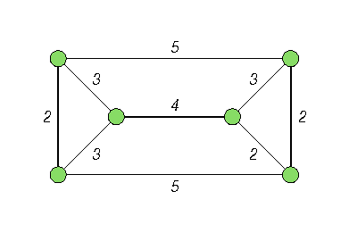
For the library matching solver, edges may be assigned with arbitrary upper capacity bounds so that both f-factors and b-matchings are covered. It is possible to determine maximum matchings and minimum cost perfect matchings, even with specifying differing lower and upper node degree bounds.
For an undirected graph and some node set T with even cardinality, a T-join is a subgraph such that exactly the nodes in T have odd degree. This model covers several other optimization problems:
While the first two problems are indeed solved in the library by application of a T-join method, the 1-matching problem cannot be solved this way since it self forms part of the T-join method. When optimizing T-joins explicitly, the odd nodes (terminal nodes) are specified by the node demand labels.
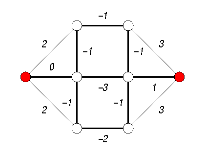
The following figure shows a subgraph with two odd nodes. In fact, it is a minimum T-join for this odd node set. This example shows that a T-join for a 2-element node set T is a path only in certain circumstances. To this end, a sufficient condition is that no negative length cycles exist:
